- Introduction
- Brains
- Simple transformation
- A simple model
- A simple atlas
- Flattening the world
- Flattening the cortex
- Pictures in support
- Conclusions
- References
Introduction
We generally concern ourselves with the micro world of LWS-N, which can be entered through reference 1. Here we concern ourselves with the macro world of brains more generally, in particular with the business of comparing or adding up the different pictures of brains we get from scanners, with this adding up and comparing depending critically on place, as we will explain in what follows. We restrict ourselves to MRI scanners, the ones which are noisy and are apt to induce claustrophobia, and which are conveniently introduced at reference 2.
We start by observing that these scanners are not only noisy from the point of view of the subjects who are being imaged, who are inside them, but the resultant images are very noisy, which means that for some purposes it is convenient to be able to add the signals from a number of scans to produce a composite signal, an adding up which is done by place. One adds up all the signals for each place in the brain. This is just one reason for wanting to know about place.
Another is the desire to communicate results between all the members of a team or between teams scattered around the country, scattered around the world even. This is much easier if one can say things like ‘in such and such circumstances, the signal at such and such a place was blah’. Again, one is interested here in what we might mean by place. Communication also leads to visualisation, and two dimensional visualisations are often convenient, visualisations which may well involve place too. How do we make such visualisations and how do we put places on them?
Another is demographic or statistical. If for population A the signal is X and for population B the signal is Y, we can look at the populations A and B and speculate about why the signals are different. We might be able to demonstrate correlations with this or that feature of the population. And to do this, once again we need place in order to describe the signal.
In the same way, if for person A the signal is X and for person B the signal is Y, we can look at persons A and B and speculate about why their signals are different.
 |
| Figure 1 |
We note in passing that the appearance of simplified graphs of this sort is very scale dependent, just as it is with the graphs you get in the financial pages of the better newspapers. Are we looking at square inches of cortex or square millimetres?
To attempt any of this, we need place, and we need place in some considerable detail, much more detail than is involved in naming, for example, the parts of a buttercup flower in a biology class at school. Which is non trivial in the context of the rather fluid surface structure of the brain, exhibited in what follows. Not to say slippery, as can be seen in our closing figure, Figure 16 below.
So this note is concerned with what we might mean by place and we start by introducing brains, mostly restricting our attention to healthy, adult, human brains.
Nothing novel here, more a marshalling of our own thoughts. Some of the prompts for those thoughts have been included among the references, for those readers who care to follow such things up.
Brains
 |
| Figure 2 |
The cerebral cortex comes in two halves, the two hemispheres, one on each side, with the gross structure of the two hemispheres being pretty much the same. Note that this is not so true of function; to some extent at least, the hemispheres do different jobs.
 |
| Figure 3 |
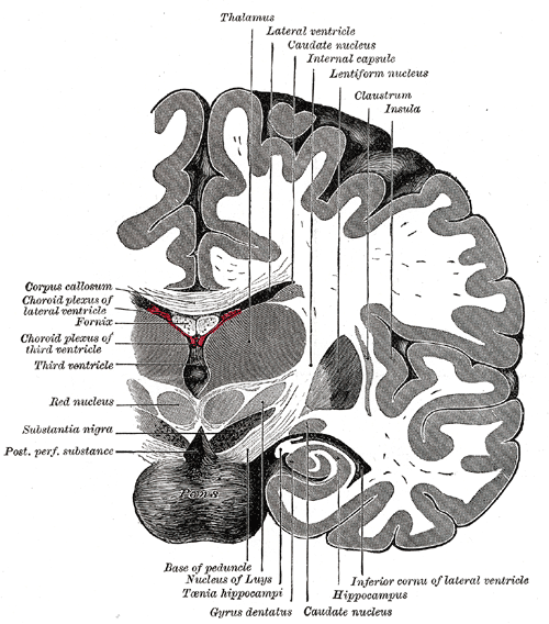 |
| Figure 4 |
Now scanners produce three dimensional images of the head, images which might be expressed as voxels, with each voxel sometimes being as small as a cubic millimetre, maybe half a million of them. So for any particular scan, of any particular person, at some particular time we can say what is going on at each point in the space for that scanner.
For the sake of simplicity, we suppose that the space for a scanner is around a cubic foot. Our problem is how to allow for the facts that the position and orientation of a head in that space is going to vary and that one head is not the same as another head. We associate to the ridges of bark on the trunks of trees: all the same general idea, and one can often tell the bark of one sort of tree from that of another sort of tree, but it there is, nevertheless, a lot of variation in detail from one tree to another.
 |
| Figure 5 |
We have also come across a small number of cases where a child is born with very little brain, but goes on to do surprisingly well. There was, for example, the case of Noah Wall , reported from Cumbria in 2016. Again, there must have been, or be, fairly drastic changes to the folding of the cortical sheet.
Simple transformations
The first thing we can do is use the landmarks on the skull to position and orientate the head, so that all our heads are at the same place and pointing the same way. This will start to bring them into alignment.
The second thing we can do is to adjust the three dimensions of the head – height, width and depth – to some standard, either taken from some particular head or from some composite or average of many heads. We can stretch and shrink our particular head to conform with the standard head. This will bring them further into alignment. The upper halves of the skulls, the brain cases, might be in quite good alignment.
But at the level of the structures visible in Figures 3 and 4 above, structures which are reasonably well conserved across populations, the alignment will not be so good. Distances between the corresponding positions of different brains are often of the order of a centimetre or more adrift – with a centimetre being a long way in terms of crossing some of the valleys of the folds shown in Figure 3, aka the sulci, as opposed to the hills, which are called the gyri – and we need to do better.
A simple model
 |
| Figure 6 |
 |
| Figure 7 |
In this figure we have put the two spheres together, added the stuff in the middle and suggested its place in the body, including in this last things like mouth, ears and eyes as well as things like legs, arms and intestines. The most conspicuous part of the brain is the shell of the cerebral cortex, here in blue and where a lot of the heavy lifting is done. The gross structure of the two halves is very much the same and the whole is encased in the hard protective shell of the cranium, roughly a sphere with a hole cut in the bottom. In the middle we have the inner brain with a lot of management functions – and in terms of evolution, mostly very old. And a lot of it conserved across related vertebrates. In between we have inner communications, linking the various sectors of the outer brain together, in particular linking the two halves (mainly via the fat bundle of nerve fibres called the corpus callosum suggested by the green arrow) and linking the outer brain to the inner brain – mostly with point-to-point connections, nothing like the structured cabling systems that computer network people talk about. Another fat bundle of nerve fibres, making up most of the brain stem and the spinal cord, links the inner brain to the body, suggested in brown below. For present purposes we have omitted the additional cerebral cortex, the cerebellum, introduced at Figure 2 above. We have also omitted the brain’s extensive blood supply, the skull and the various voids.
We allow a zona incerta where the various zones meet and where things are likely to be a bit more of a muddle under the microscope than this simple diagram would suggest. We note that, at a macroscopic level, the inner brain is a lot more complicated that the outer brain. The former has lots of readily distinguished parts, while the later is relatively homogenous, a simple sheet, just layered and folded.
A companion piece to the diagram offered at reference 4.
In what follows, we shall be mostly interested in the cortical sheet, the cerebral cortex. In particular, with mapping that sheet, a two dimensional sheet embedded in regular, three dimensional space, onto the plane.
A simple atlas
 |
| Figure 8 |
In the green, we have the standard volume of the brain as a whole and a small number of standard cortical sheets. Perhaps one spherical and one flat. There is a deformation which gets us from the cortical sheet of the standard volume to each of the standard sheets.
In the orange, we have data about the standard brain, expressed in the form of voxel values for volumes and pixel values for sheets, borrowing here the jargon used for MRI and pictures respectively.
In the blue, we have labels for our standard brain, labels which will apply to some or all of the standard objects.
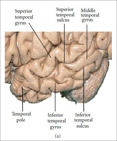
- Anatomy. Major landmarks such as the temporal and frontal poles. Bone, gray matter, white matter, voids, other. The sort of stuff that you can pick out, for example, from Figure 2 above
- Gyri and sulci. The sort of stuff that you can pick our from Figure 3 above
- Histology. The sort of thing for which, for the moment at least, one needs to take thin sections, stain them and then look at them through a microscope. Mix of cells, arrangement of layers
- Areas. The atlas knows about various previous partitions of the cortical sheet into areas, each such partition here being called an areaset (to rhyme with dataset). In particular the long lived Brodmann areas described at reference 7 and illustrated by Figure 13 below.
We note that the average area of a Brodmann area is of the order of 20 square centimetres, about four times the hypothesised area of the bit of cortex supporting LWS-N .
Things we do not do:
- Say anything about the brain’s blood supply, not insignificant in terms of the space occupied
- Attempt to put any probability on all of this, to have our standard brain say something about how likely it is that any particular feature is at any particular place, although we believe that some atlases do do this
- Attempt to define place by function rather than by structure. Which might be a way to deal with brain plasticity, the brain’s lack of respect for boundary lines drawn on the cortical sheet.
 |
| Figure 9 |
We make the reasonable assumption that the two sets of landmarks, the blue and the green in the figure above, are reasonably well aligned, so that a continuous, not very drastic deformation is possible; that the deformation is not so very deforming.
We are then in a position to describe what is going on in our particular brain in terms of the standard brain which everyone else understands.
Flattening the world
Before looking at flattening the cortical surface, we first look at the rather simpler, but well known problem, of flattening out the surface of the earth, usually for the purposes of making maps to put in books.
The first thought is of flattening out orange peel, for which reference 6 from Hawaii provides a suitable illustration, turned up by Google.
 |
| Figure 10 |
 |
| Figure 11 - with thanks to Daniel R. Strebe |
Note that the design of this projection takes the various land masses of the earth into account; it is land mass sensitive. It also involves less cuts than were needed for the orange peel solution.
Flattening the cortex
So how are we going to do this for the thin, folded sheet of cerebral cortex, around 2,000 square centimetres of it taking the two hemispheres of the brain together? Bearing in mind that mapping this much folded brain onto the flat pages of an atlas is a rather more complicated problem than mapping of the surface of the earth, a problem which has, as we have seen, generated lots of interesting solutions over the years.
 |
| Figure 12 |
With Mollweide being an astronomer, interested in mapping the night sky, another hemisphere.
 |
| Figure 13 |
 |
| Figure 14 |
Pictures in support
 |
| Figure 15 |
 |
| Figure 16 |
And we finally close with the comment that the arrival of scanners has meant that we can make a lot of progress without needing to invade brains in the way of Figure 16 – alive or dead – to do it. A big change for the better.
Conclusions
We have tried to give something of the flavour of defining place in the brain and the use of those places in making map and in comparing one brain with another.
References
Reference 1: https://psmv3.blogspot.com/2018/05/an-update-on-seeing-red-rectangles.html.
Reference 2: https://en.wikipedia.org/wiki/Functional_magnetic_resonance_imaging.
Reference 3: Anatomy of the Temporal Lobe - J.A.Kiernan – 2012.
Reference 4: http://psmv3.blogspot.com/2017/04/its-chips-life.html.
Reference 5: The cerebral sulci and gyri - Guilherme Carvalhal Ribas – 2010.
Reference 6: https://manoa.hawaii.edu/sealearning/.
Reference 7: Centenary of Brodmann’s map — conception and fate - Karl Zilles and Katrin Amunts – 2010.
Reference 8: Hemispherically-Unified Surface Maps of Human Cerebral Cortex: Reliability and Hemispheric Asymmetries - Xiaojian Kang, Timothy J. Herron, Anthony D. Cate, E. William Yund, David L. Woods – 2012.
Reference 9: http://imaging.mrc-cbu.cam.ac.uk/imaging/BrodmannAreas.
Reference 10: Cortical cell and neuron density estimates in one chimpanzee hemisphere - Christine E. Collins and others – 2016.
Reference 11: Anatomy of the Temporal Lobe - J.A.Kiernan – 2012.
No comments:
Post a Comment